TikZ diagrams with R: A Normal probability distribution function

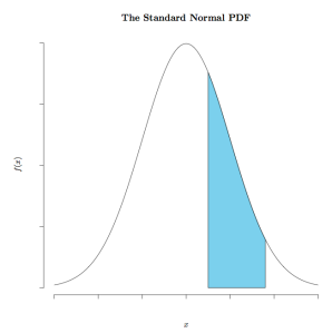
You may have seen an earlier post where I went through some examples of how to create a normal distribution in LaTeX using TikZ. In this post, I will show a different way to accomplish a similar result using R and the package tikzDevice().

tikzDevice() is an R package that outputs any image from R as TikZ code in a .tex file. In order to include the outputted .tex file in you LaTeX document, you need to do two things:

• add \usepackage{tikz} in the preamble to your LaTeX document.
• add \include{normal_pdf} where you’d like your image (after you’ve created and outputted normal_pdf.tex from R, as shown below).

R:

# load tikzDevice package
require(tikzDevice)

# Choose boundaries to be shaded in blue
a = 0.5
b = 1.8

# creates x & y boundaries based on a and b parameters
x.val <- c(a,seq(a,b,0.01),b) 
y.val <- c(0,dnorm(seq(a,b,0.01)),0)

# choose the name and location for your .tex file
# it should be the same directory as your latex document
tikz( '/Users/kevingoulding/latex_documents/thesis/normal_pdf.tex' )

# plots a normal distribution curve
curve(dnorm(x,0,1),xlim=c(-3,3),main='The Standard Normal PDF',
	xlab = '$x$', ylab = '$f(x)$',
	frame.plot = FALSE, axes = FALSE)

# shades in a polygon underneath curve
polygon(x.val,y.val,col='skyblue')

# creates blank axes
Axis(side=1, labels=FALSE)
Axis(side=2, labels=FALSE)

# must turn device off to complete .tex file
dev.off()

Tags: LaTeX, plots, R, TikZ