Differences-in-Differences estimation in R and Stata

{ a.k.a. Difference-in-Difference, Difference-in-Differences,DD, DID, D-I-D. }

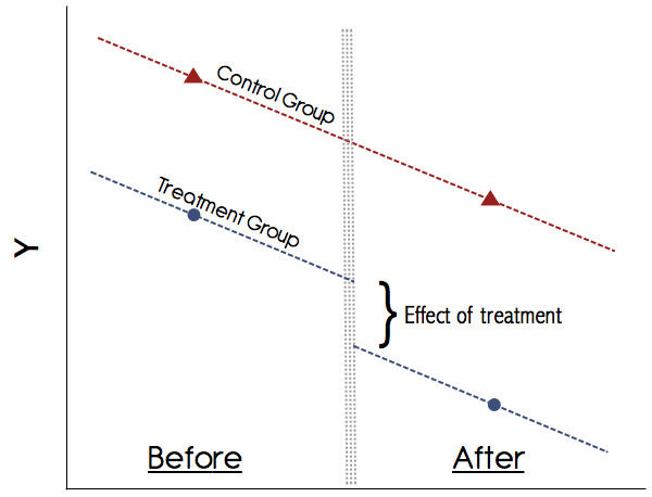
DID estimation uses four data points to deduce the impact of a policy change or some other shock (a.k.a. treatment) on the treated population: the effect of the treatment on the treated.  The structure of the experiment implies that the treatment group and control group have similar characteristics and are trending in the same way over time.  This means that the counterfactual (unobserved scenario) is that had the treated group not received treatment, its mean value would be the same distance from the control group in the second period.  See the diagram below; the four data points are the observed mean (average) of each group. These are the only data points necessary to calculate the effect of the treatment on the treated.  The dotted lines represent the trend that is not observed by the researcher.  Notice that although the means are different, they both have the same time trend (i.e. slope).

For a more thorough work through of the effect of the Earned Income Tax Credit on female employment, see an earlier post of mine:

Calculate the D-I-D Estimate of the Treatment Effect

We will now use R and Stata to calculate the unconditional difference-in-difference estimates of the effect of the 1993 EITC expansion on employment of single women.

R:

# Load the foreign package
require(foreign)

# Import data from web site

require(foreign)

# update: first download the file eitc.dta from this link:
# https://docs.google.com/open?id=0B0iAUHM7ljQ1cUZvRWxjUmpfVXM
# Then import from your hard drive:
eitc = read.dta("C:/link/to/my/download/folder/eitc.dta")

# Create two additional dummy variables to indicate before/after
# and treatment/control groups.

# the EITC went into effect in the year 1994
eitc$post93 = as.numeric(eitc$year >= 1994)

# The EITC only affects women with at least one child, so the
# treatment group will be all women with children.
eitc$anykids = as.numeric(eitc$children >= 1)

# Compute the four data points needed in the DID calculation:
a = sapply(subset(eitc, post93 == 0 & anykids == 0, select=work), mean)
b = sapply(subset(eitc, post93 == 0 & anykids == 1, select=work), mean)
c = sapply(subset(eitc, post93 == 1 & anykids == 0, select=work), mean)
d = sapply(subset(eitc, post93 == 1 & anykids == 1, select=work), mean)

# Compute the effect of the EITC on the employment of women with children:
(d-c)-(b-a)

The result is the width of the “shift” shown in the diagram above.

STATA:

cd "C:\DATA\Econ 562\homework"
use eitc, clear

gen anykids = (children >= 1)
gen post93 = (year >= 1994)

mean work if post93==0 & anykids==0     /* value 1 */
mean work if post93==0 & anykids==1     /* value 2 */
mean work if post93==1 & anykids==0     /* value 3 */
mean work if post93==1 & anykids==1     /* value 4 */

Then you must do the calculation by hand (shown on the last line of the R code).
(value 4 – value 3) – (value 2 – value 1)

Run a simple D-I-D Regression

Now we will run a regression to estimate the conditional difference-in-difference estimate of the effect of the Earned Income Tax Credit on “work”, using all women with children as the treatment group. This is exactly the same as what we did manually above, now using ordinary least squares. The regression equation is as follows:

Where is the white noise error term, and is the effect of the treatment on the treated — the shift shown in the diagram. To be clear, the coefficient on is the value we are interested in (i.e., ).

R:

eitc$p93kids.interaction = eitc$post93*eitc$anykids
reg1 = lm(work ~ post93 + anykids + p93kids.interaction, data = eitc)
summary(reg1)

The coefficient estimate on p93kids.interaction should match the value calculated manually above.

STATA:

gen interaction = post93*anykids
reg work post93 anykids interaction

Tags: R, STATA